3D astigmatism tool
This page describes the Astigmatism 3D tool, used to calibrate an axial astigmatism model and estimate the axial position (Z) from PSF widths (Sigma X / Sigma Y).
Launch
Open a terminal or command prompt (
PowerShellon Windows) in the folder where you extracted the project files. Example forC:\palm-tracer. Open the terminal and type the following command:cd C:\palm_tracer, then press Enter.Make sure the virtual environment is activated if you are using one.
Launch Napari with the command:
napari
Note
If you did not create a virtual environment, Napari can be launched from anywhere.
Launch the tool in Napari:
Interface organization
The tool is organized into two tabs corresponding to the two main steps of the workflow.
- The interface is organized into two tabs, corresponding to the two classical steps of the astigmatic workflow:
Compute Model: calibration of the astigmatism model from calibrated data
Estimate Z: estimation of the axial position from an existing model.
The right part of the window continuously displays a visualization of the current astigmatic model (Sigma X and Sigma Y curves as a function of Z). You can click the camera icon (📷) above the graph to directly save a PNG image.
Tab 1: Model computation. |
Tab 2: Axial position estimation (Z) |
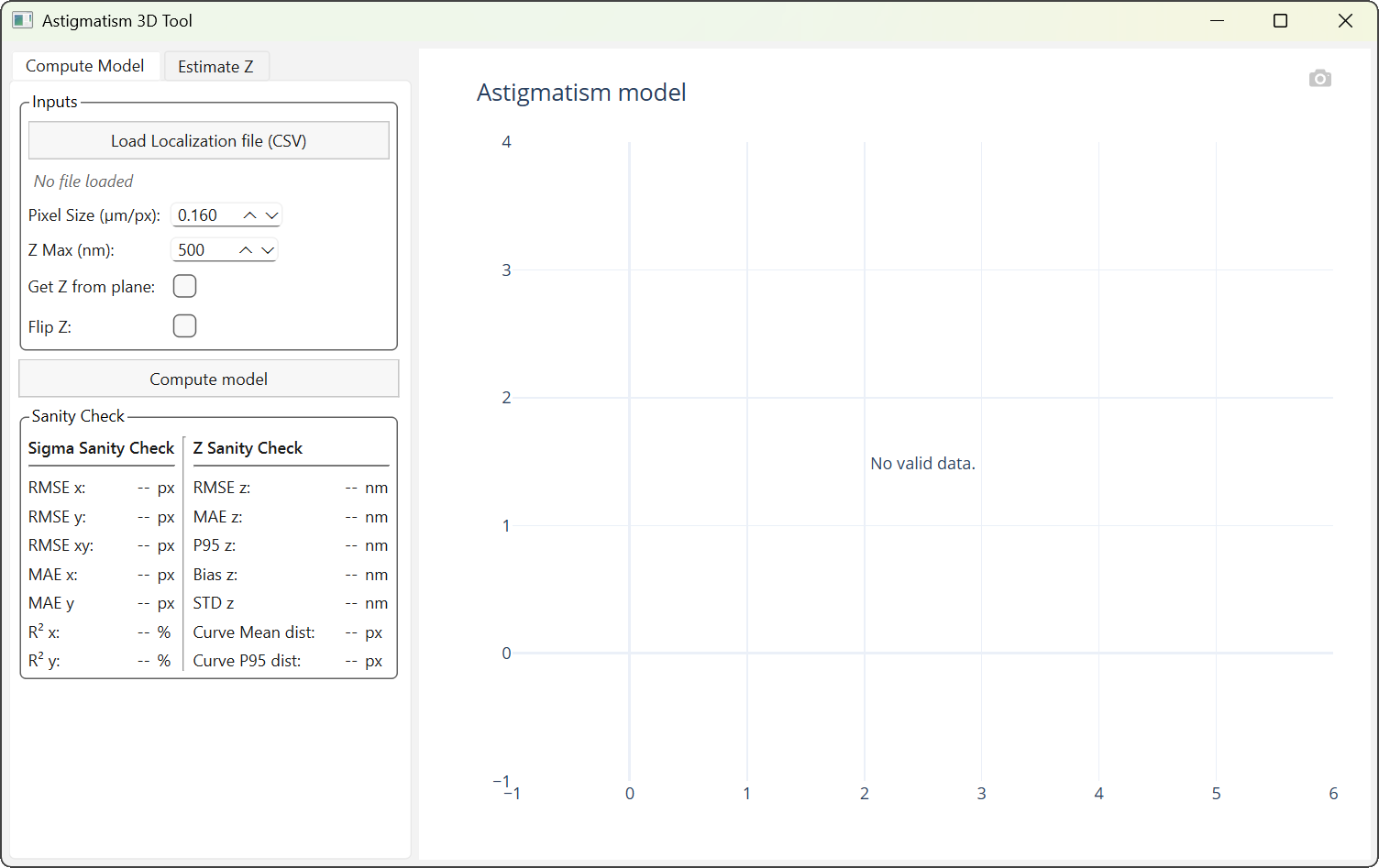
Model computation
This tab allows computing an astigmatism model from a set of Z-calibrated localizations.
- After loading a CSV file containing at least the columns
Sigma X,Sigma Y, andZ, the following parameters can be adjusted: the pixel size (µm/px),
the maximum Z value,
optional reconstruction of Z from planes,
inversion of the Z sign.
After loading, the file name appears below the corresponding button. Hovering over the name with the mouse cursor displays the full file path.
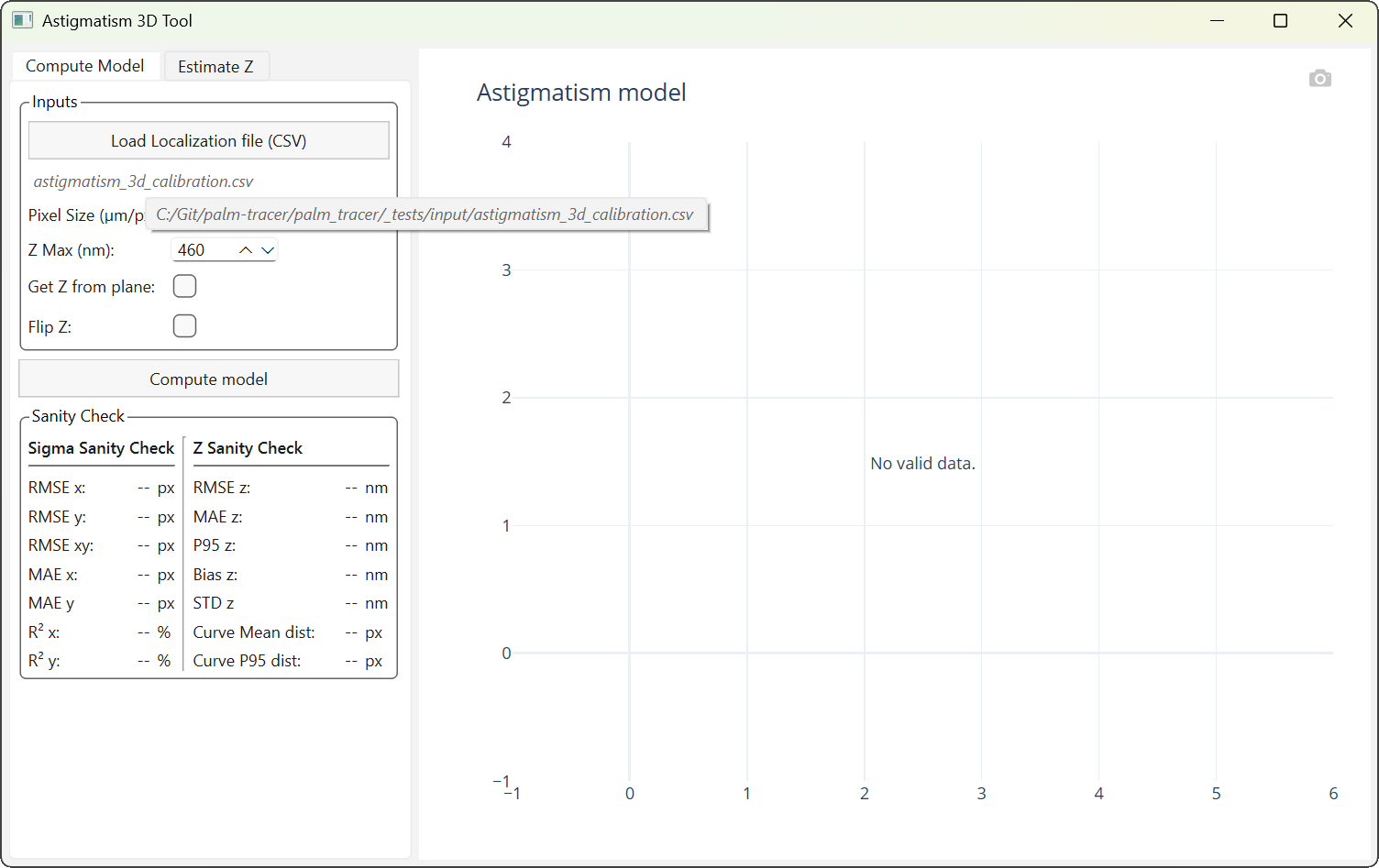
Display of the full file path.
If Z is not calibrated, planes are used (therefore a Plane column is required) to fill the Z column. You must enable the Get Z from plane option and specify the absolute maximum Z value (Z Max) in nanometers to reconstruct Z over the interval [-Z Max; +Z Max].
Important
The increasing or decreasing order of planes cannot be detected automatically. A Z inversion may be required depending on the experimental convention.
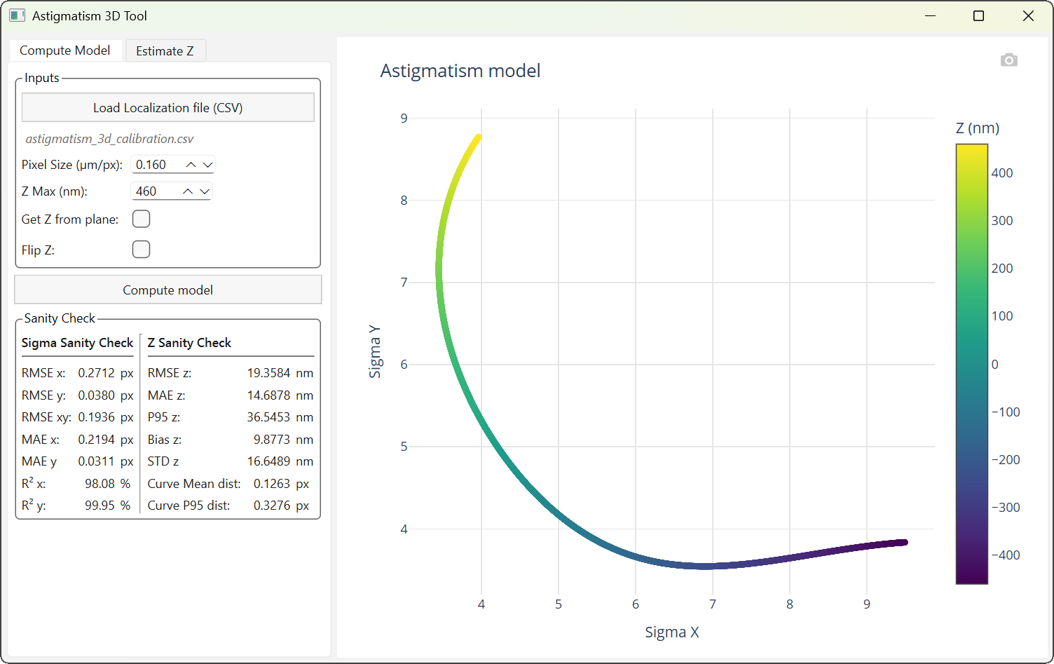
Clicking the Compute model button starts the computation. This generates a file named astigmatism_3d_model.csv in the calibration file directory.
Consistency indicators (Sanity Check) are automatically updated, and the model is displayed in the visualization area.
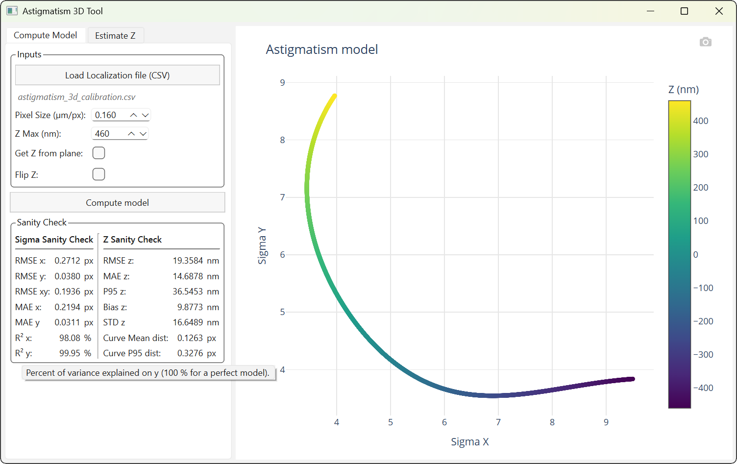
3D astigmatism model computation interface.
The Sanity Check area provides simple indicators to quickly assess the quality of the model.
The left column groups metrics related to PSF widths (RMSE, MAE, R² on Sigma X and Sigma Y). The right column concerns the axial consistency of the model (Z errors, bias, dispersion, and distance to the curve).
These values allow quickly detecting an inconsistent model, a Z inversion, or a poorly defined axial range. As with file names, hovering with the mouse cursor provides an explanation for each metric.
Important
The increasing or decreasing order of planes cannot be detected automatically. A Z inversion may be required depending on the experimental convention.
Display of explanations for sanity check metrics.
Note
An ideal calibration file has an odd number of rows (to have the central row with Z=0) linearly distributed over the interval [-Z Max; +Z Max]. The spacing between planes should be as small as possible to ensure model reliability. Irregularities in plane distribution (non-uniform spacing, interval not centered at 0, etc.) cannot be automatically handled. In such cases, it is recommended to fill the Z column beforehand.
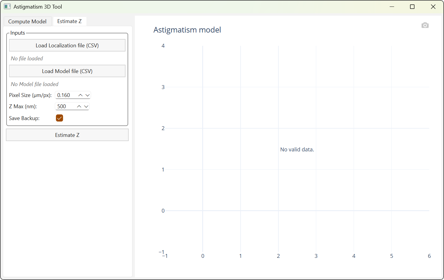
Axial position estimation (Z)
This tab allows estimating the axial position for a given localization file containing at least the columns Sigma X, Sigma Y, and Z, using an existing astigmatism model.
Pixel size and axial range parameters must be consistent with those used during model calibration.
If the Save Backup option is enabled, a copy of the original file is saved before updating the Z column.
Clicking the Estimate Z button starts the estimation. The CSV file is then rewritten at the same location, with the Z column updated.
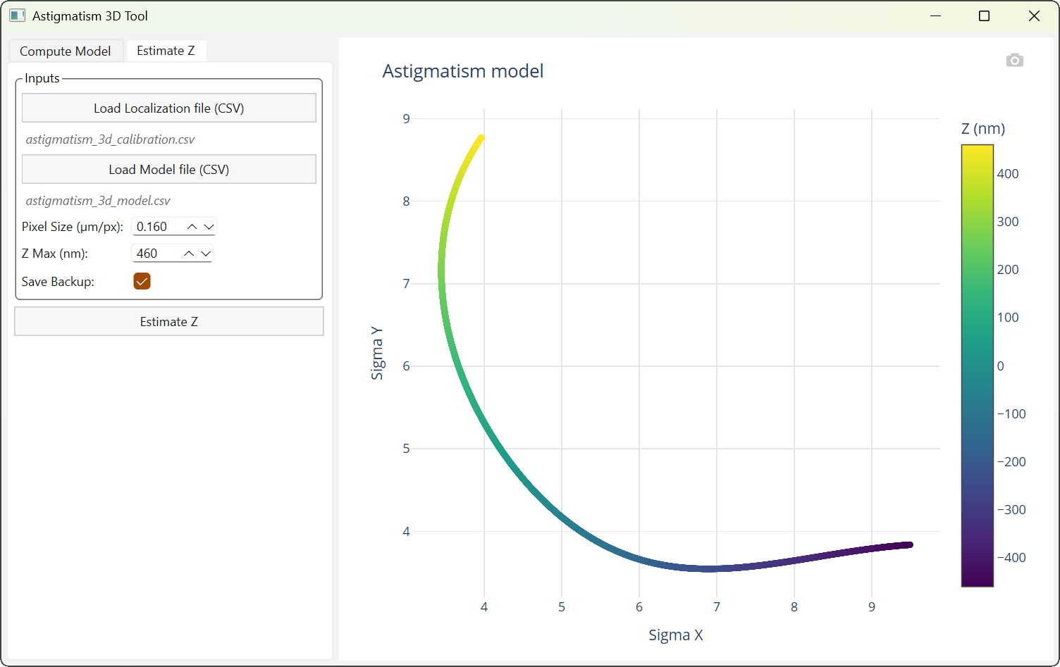
Axial position estimation (Z) interface.